Mathematics

Recently I have been taking some notes on the classic paper by Dijkgraaf and Witten on topological field theories with finite gauge group (part I of that series). As tends to happen, when you read such a paper you get spun off in all kinds of directions, and notice things you really do not understand. In my case, this thing was the importance of torsion in homology. As I mused here, the root of this problem is that physicists use differential forms to define geometric quantities like the action – which are naturally elements in de Rham cohomology, and take values in $\mathbb{R}$ . However, when you want to start thinking about the topology of the underlying manifolds, you need to use concepts coming from integer (co-)homology. In the case of Chern-Simons theory, we need to know under what conditions we can extend a vector bundle from a 3-chain to a 4-chain, which is a question rooted in topology, and thus requires integer homology to answer.

I first learned homology from Hatcher (like so many of us…). I read all of the sections of homology, then read “cohomology is the dual of homology”, stopped reading and started learning about de Rham cohomology. I did this because I am a dummy (physicist). When you think about the “important lessons” from homology, it’s easy to answer something like “homology tells you the cellular decomposition of a space”, because that concept easily maps into de Rham cohomology via Poincare duality. Of course, that’s only because you’ve forgotten about torsion!

Generally, torsion elements of a group are those which have finite order. Homology groups can be written as

$H_i(M)=\mathbb{Z}_{p_1}\oplus...\oplus \mathbb{Z}_{p_q}\oplus \mathbb{Z}^n$

where we have $q$ torsion elements of orders $\{p_i\}$ , and $n$ generators of the infinite cyclic parts ( $n$ would be the Betti number). When you calculate the homology groups of nice examples like spheres and tori, you might not notice torsion. However, you see it pretty quickly after that (see an earlier post for an example on $\mathbb{R}P^2$ ). So who cares about torsion? How can we detect torsion and how can it affect something like the action in a physical theory?

I found a nice answer after reading a paper from Daniel S. Freed, Determinants, Torsion, and Strings (1986). Besides having a very nice explanation of what I am talking about, he has a rather amusing attitude about fact that he has to to be the one to tell physicists about torsion: “The author faces here the unenviable task of explaining these ideas, which perhaps are not completely standard in mathematics, to an audience partly composed of (brave) physicists…” I will elaborate on his short discussion here, and fill in a few gaps here and there since I have room to do so. His audience was (brave) physicists – mine will be myself approximately 2 weeks ago. At that time I knew things about de Rham cohomology and singular homology, but all I knew about torsion was that somehow got in the way of Poincare duality…

Given an abelian group $G$ , we have a subgroup $Tor(G)$ of the torsion elements (notice the abelian assumption is crucial here. For instance, torsion elements of $\mathbb{Z}_2$ in the free product $\mathbb{Z}_2\star\mathbb{Z}_2$ do not have finite order. Thanks to F. Cohen for pointing this out to me) . There is an exact sequence

$0\to Tor(G)\xrightarrow{i} G\xrightarrow{j} Free(G) \to 0$

where $i$ is the inclusion (an exact sequence means the image of each map is the kernel of the next). $Free(G)$ is the “free part of G”, and since $Im(i)=Ker(j)$ we can explicitly define $j$ as

$j(g)=\left\{\begin{aligned}1~&~g\in Tor(G)\\g~&~\mbox{otherwise}\end{aligned}\right.$

By the first isomorphism theorem, we know that the last group is: $Free(G)\cong G/Tor(G)$ . Now we specialize the discussion to $G=H^k(M)$ for smooth manifold $M$ (Freed calls $M$ a “reasonable space” – but we are physicists so all reasonable spaces are smooth…). Also notice that if I leave coefficients out of $H^k(M;\mathbb{Z})$ , I am implying integers.

So in physics, integrals of these classes are actions – so let’s evaluate the integral of the free part of a cohomology class $c^{free}\in Free(H^k(M))\cong Hom(Free H_k(M),\mathbb{Z})$ (the isomorphism is the definition of the cohomology classes as dual to the homology classes). This cohomology class is represented by a closed 1-form $\gamma\in \Omega^k(M)$ (which is also an element in the de Rham complex). Now the usual set up for computing the integral of a form on a manifold follows: a fundamental class on $M$ is a pair $(\Delta^p,f)$ where $\Delta^p$ is a simplex in $\mathbb{R}^p$ and $f:U\subset \mathbb{R}^p\to M$ smooth. The fundamental class can be represented by a homology class $[M]\in H_k(M)$ and we have the pairing

$\langle c,[M]\rangle = \int_M f^*(\gamma)$

(If you are not familiar with this pairing, you can take it as a definition). The brackets give us a map $H^k(M)\otimes H_k(M)\to \mathbb{Z}$ , which is an integer since the form $\gamma$ is the representation of an integer class.

Now consider what happens if we integrate over a torsion element. We need the following result from the Universal Coefficient Theorem (which deserves it’s own post here at some point)

$Tor(H^k(M))\cong Tor(H_{k-1}(M))$

So we start with a torsion class $[p]\in H_{k-1}(M)$ . Writing the groups additively (and assuming that our brains can think outside of the group structure and multiply elements…) we have $k[p]=0$ for $k\in\mathbb{Z}$ . Now pick a chain $q\in C_k(M)$ such that $\partial q=kp$ , where I write $p\in C_{k-1}(M)$ (the chain, not the class). Now $p$ is an integer chain so $\partial (q/k)$ is an integer chain too. However, this does not mean $q/k$ is necessarily integer any more – $q/k$ has coefficients in $\mathbb{Q}$ (rational numbers, specifically those of the form $m/p$ for $m\in \mathbb{Z}$ ). Now denote the chain $\bar{q}$ as the form $q/k$ with the “coefficients reduced”.

(This means that for every coefficient $m/k$ of $q$ , we “subtract off all the integer parts”. If $m<k$ then $m/k<1$ and we are done. If $rk>m>k,~r\in\mathbb{Z}$ , write $l=m-rk$ and:

$\frac{m}{k}=\frac{rk+l}{k}=r+\frac{l}{k}$ .

Now replace the coefficient $m/k$ with $l/k<1$ . No one is going to read this garbage, right…?)

In any case, this means $\bar{q}$ is closed – we have basically replaced $q/k\to rq + \bar{q}$ with $r\in\mathbb{Z}$ , and “there is no way” (go away mathematicians) that the rational numbers in $\bar{q}$ will add up to be an integer. Thus, $\partial \bar{q}$ must vanish, and

$[\bar{q}]\in H_k(M;\mathbb{Z}/k)$ .

Now since this is an element of $k$ -homology, we can evaluate it on the $k$ -class c from above to get

$\langle c,[\bar{q}]\rangle \in \mathbb{Z}/k$

So the point is that integration on integer cohomology classes breaks into $\mathbb{Z}$ on the free part and $\mathbb{Q}$ on the torsion part. These are related to topological structures and invariants, which is why they are important in topological quantum field theories, like what I am interested in right now. The major lesson here is that since the integration on forms detects the difference between torsion and non-torsion elements, they actually hold some importance for physics. However, at this level it appears that this is true only when the forms are restricted to be integral.

“We could lick gravity, but sometimes the paperwork is overwhelming”

-Wernher von Braun

Dr. von Braun (yes, that Dr. von Braun) was not just being a smartass German; this is a major stumbling block. General Relativity is a beautiful theory which is incredibly hard to use gracefully. There are several reasons, and I will just highlight two of them.

Spacetime is four-dimensional. The lengths between any two points in a four-dimensional space is given by a (usually symmetric) 4×4 matrix called the metric. A symmetric 4×4 matrix has 10 independent components. The Einstein field equations tells us how each of these 10 components evolve – via a set of 10 nonlinear partial differential equations. To find solutions to these equations (and thus determine the geometry of spacetime), we often exploit symmetries of the problem. For instance, in cosmology we assume spacetime is homogenous (the same at every point in space) and isotropic (the same in every direction), which reduces the number of unknown parameters of the metric from 10 to 1 (the scale factor). There is no general solution for the full Einstein equations.

General Relativity is background independent. I could talk all day about this, but this is the feature which separates GR from all other physical theories (electromagnetism for instance, and all quantum everything). This means the theory is completely self-contained – matter generates spacetime curvature and spacetime curvature acts like matter. Take electrodynamics; photons and electrons travel in a spacetime background, but do not change the spacetime background. That GR has this feature certainly suggests that it is “more fundamental” than other classical theories which still require humans to put in some features of the theory by hand. This makes the 10 components of the metric very dependent on each other (highly coupled), but also it means there is no natural way to do a perturbative expansion. Which is not to say linearized gravity (small changes to the gravitational field which occur on a fixed background) is not useful – that’s where most of what we know about gravitational waves comes from – but when you linearize gravity you break its background independence. This changes the fundamental structure of the theory and makes it behave like the others – which it doesn’t. There is no known way to study small changes to the gravitational field and preserve its background independence.

That’s all to say that General Relativity is hard because geometry in four dimensions is hard. One of the major topics of my work is to try and find some simplifications of the geometry to learn things about the physics. A key mathematical tool is:

Definition A covering space is a space $M$ together with a surjective map $\pi: M \rightarrow B$ such that for every $x\in B$ there is a neighborhood $U$ of $x$ such

$\pi^{-1}(U)=V_1\cup V_2...\cup V_n$

where each $V_i$ is an open set in $M$ . For every covering map $n$ is a constant integer, and we say that $M$ is an $n$ -sheeted cover.

Wait not that. This:

Definition A branched covering space is a space $M$ together with a surjective map $\pi: M \rightarrow B$ such that outside of a finite set $R\subset B$ , $M$ is a covering space.

The set $R$ is called the branch locus, and over the branch locus some of the sheets “collide”, so that there are now $m<n$ inverse images of the covering map. An illustration may be more helpful:

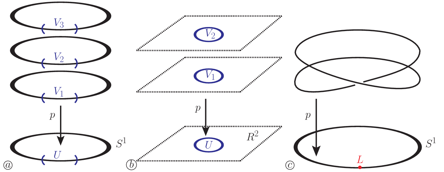
In this figure, (a) and (b) are examples of unbranched covering spaces, whereas (c) is a branched covering space of the circle with branch locus the point $L$ . The picture makes it seem like the covers are “crossing” each other, but it’s more accurate to say they are “glued together” in some specific manner. In fact, every singular point is described locally via coordinates $z^n$ for an $n$ -fold cover which is why this is very hard to draw in 3 dimensions. The details of why that produces a smooth manifold (as opposed to a figure 8 space, like what you’re probably thinking) are a bit too much for this post.

The reason all this belongs on my website is the following classical result:

Alexander’s Theorem: Any compact smooth n-manifold ( $n > 2$ ) can be represented as a covering space of the n-sphere branched over an $(n-2)$ -complex.

That’s a lot of manifolds! What is most interesting is that since branched covering spaces are just copies of the base space intersecting in some funny ways (like the figure), this means we can represent arbitrary compact, smooth n-manifolds as spheres which have been glued together. This greatly reduces the possibility complexity, particularly when you start thinking about dimensions 3 and 4. The reason this works can be found in the original proof: you start with a triangulation of an arbitrary 3-manifold, and a map from the triangulation to the triangulation of a sphere. This triangulation consists of two 3-complexes, one which contains the point at infinity and one which does not. By just making sure the orientations all work out, one can map each complex in the manifold to one of the two in the sphere, with a map that is p to 1 everywhere but at the vertices and edges of the complex. This argument can be easily extended to higher dimensions.

In fact, this is the first of a whole set of similar results. For instance, you can realize any closed 3-manifold over one specific knot, and you can realize 4-manifolds not just over 2-complexes but over smooth embedded surfaces (provided the number of covers is at least 4). I won’t go into where these specific results come from, but suffice to say it affords lots of opportunities for interesting model-building in physics – essentially by reparametrizing the degrees of freedom of the model in terms of this geometric and topological information.

In the next post I will present one example of an application which I have worked on – a reparametrization of the gravitational field which I make needlessly complicated and find some interesting connections to spinors and cosmic strings…

Christopher Duston's Home

Mathematical Physics and Propaganda

Torsion for Dummies (Physicists)

Representing Spacetime as a Branched Covering Space