In this final post I will explain the two primary examples found in the Dijkgraaf and Witten paper, and give some concluding remarks regarding my original interest in this topic – the application to loop quantum gravity.
Example Calculations, Continued.
The first example from the paper is  (2-sphere with 3 punctures times 1-sphere), which can be used to generate many complicated examples. First we need a representation of this space as a simplex:
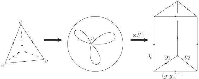
The first picture shows that  can be represented as a 2-complex with the three vertices identified. Taking the product of this with the circle gives us the final image. This can be decomposed into 3 simplices, as shown:
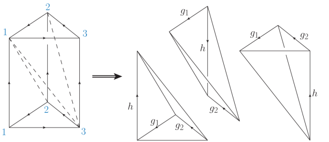
This is certainly confusing, since not only is the top and bottom identified, but all the vertices are being identified (if you recall in the last post orientation was an issue – that is not a problem here due to how this gluing is happening. Just stare at it long enough and it should seem obvious, even if it’s not). In any case, this is the easiest decomposition into tetrahedrons (3D figures with four triangular faces). If the first simplex has positive orientation, the middle one must have negative orientation since their faces are in contact – counterclockwise on the faces of the first results in clockwise on the middle. The third one is again positive, and using the order of the vertices we find the action to be

It’s a messy but very doable calculation to show that  – it’s a cocycle. In addition, we should check that under
  we get
  for some 1-cocycle
  .. This will get a bit messy as well, but it has at least one subtly so I’ll do it.

To cancel out a bunch of those terms I have used the fact that the  s are in the stabilizer subgroup of the
  – so
– so  . This can also be seen from the simplicial complex representation above. So we see that the transformation works if
  is the 1-cocyle which transforms
  , because
  is a 2-cocycle so that:

The first equality comes from the definition of a coboundary, and the second is using the definition of the 1-form  . This matches the expression above.
The next example we will do is  (the three torus). This can be represented as the cube with opposite sides identified, which splits into 6 simplices, a pair of which is shown below.
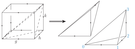
Each pair of these simplices have differential orientation and order of edges. The ones I have shown contribute  , and by permutation it’s pretty easy to see the action is
As stated above, we can generate a higher-genus surface with the manifold ; in the case of the 3-torus it is easy to see that it takes two to make (just cut the cube along a diagonal and you get a prism). Therefore we can write the action in terms of the 2-cocycles  .
.
TQFT and Loop Quantum Gravity
In loop quantum gravity we don’t have a lattice but rather a graph – which is something like an irregular lattice. The fields live in  , and in a 2009 paper, Bianchi constructed something which (at least superficially) looks very much like a TFT by considering the moduli space of flat connections. However, the actual topological character is rather hidden in this approach, and in fact in all of the standard approaches to LQG (BF theory, etc). This is where the motivation for topspin networks comes from – you can read more about that elsewhere on this site. The end result of the incorporation of topspin networks is additional
  labels on the spin networks – which turns LQG into something resembling a gauge theory with finite gauge group on an irregular lattice. The idea is to construct the partition function for a TQFT associated to a topspin network and use it to measure the topological contribution to the correlation function, which is a topic of hot research right now. In addition, this should make the rather tenuous connection between group field theory and LQG more clear.
So…watch out on the archive!


Wow, love this article beautiful work. Thanks.
Pingback: Background independence in a nutshell: the dynamics of a tetrahedron by Rovelli et al | quantumtetrahedron
Pingback: The Quantum Tetrahedron and the 6j symbol in quantum gravity | quantumtetrahedron
Pingback: The length operator in Loop Quantum Gravity by Bianchi | quantumtetrahedron
Pingback: Linking covariant and canonical LQG: new solutions to the Euclidean Scalar Constraint by Alesci, Thiemann, and Zipfel | quantumtetrahedron
Pingback: Spin-Foams for All Loop Quantum Gravity by Kaminski ,Kisielowski and Lewandowski | quantumtetrahedron